GNSS Multipath Analysis

In short

gnssmultipath is an end-to-end Python toolkit for quality control of GNSS measurements, with a particular focus on quantifying the code multipath effect for every signal and every constellation (GPS, GLONASS, Galileo and BeiDou) present in a RINEX observation file. From a single observation file plus an ephemeris source it produces multipath and ionospheric-delay time series, RMS statistics, cycle-slip diagnostics, SNR plots, az/el heatmaps and a full text/CSV report — and it can also estimate the receiver position by least-squares from the pseudoranges.

The software reads observations and ephemerides directly, with no external GNSS toolbox required:

RINEX observation files: v2.xx, v3.xx and v4.xx
RINEX navigation files (broadcast ephemerides): v2.xx, v3.xx and v4.xx, including the new RINEX 4 message types (GPS LNAV, GLONASS FDMA, Galileo I/F/INAV-FNAV, BeiDou D1/D2).
SP3 files (precise satellite coordinates): SP3-c and SP3-d are interpolated to the observation epochs using Neville's algorithm.

Introduction

GNSS Multipath Analysis is a software tool for analyzing the multipath effect on Global Navigation Satellite Systems (GNSS). The core functionality is based on the MATLAB software GNSS_Receiver_QC_2020, but has been adapted to Python and includes additional features. A considerable part of the results has been validated by comparing the results with estimates from RTKLIB. This software will be further developed, and feedback and suggestions are therefore gratefully received. Don't hesitate to report if you find bugs or missing functionality. Either by e-mail or by raising an issue here in GitHub. Contributions are also welcome!

Features

Estimates the code multipath for all GNSS systems (GPS, GLONASS, Galileo, and BeiDou).
Estimates the code multipath for all available signals/codes in the RINEX file.
Provides statistics on the total number of cycle slips detected (using both ionospheric residuals and code-phase differences).
Supports both RINEX navigation files (broadcast ephemerides) and SP3 files (precise ephemerides).
Supports RINEX v2.xx, v3.xx, and v4.xx observation files
Supports RINEX v3.xx and v4.xx navigation files (including RINEX 4 message types: GPS LNAV, GLONASS FDMA, Galileo INAV/FNAV/IFNV, BeiDou D1/D2/D1D2).
Generates various plots, including:
- Ionospheric delay over time and zenith-mapped ionospheric delay (combined).
- The multipath effect plotted against time and elevation angle (combined).
- Bar plot showing multipath RMSE for each signal and system.
- Polar plot of the multipath effect and Signal-to-Noise Ratio (SNR).
- Polar plots of SNR and multipath.
- Polar plot of each observed satellite in the system.
- SNR versus time/elevation.
- Azimuth-vs-elevation heatmaps summarizing multipath and C/N₀ across all satellites (combined and per-system).
Extracts GLONASS FCN from RINEX navigation files.
Detects cycle slips and estimates the multipath effect.
Exports results to CSV and a Python dictionary as a Pickle (both compressed and uncompressed formats are supported).
Allows selection of specific navigation systems and signal bands for analysis.
Includes a built-in CDDIS downloader for fetching GNSS data (navigation, observation, and SP3 files) directly from NASA's CDDIS archive via FTPS.
Estimate the approximate position of the receiver using pseudoranges from the RINEX observation file.
- Supports both SP3 and RINEX navigation files.
- The software will estimate the receiver's position if it is not provided in the header of the RINEX observation file.
- Supports user-defined Coordinate Reference System (CRS). The estimated coordinates can be delivered in the desired CRS.
- Calculates statistical measures for the estimated position, including:
  - Residuals
  - Sum of Squared Errors (SSE)
  - Cofactor matrix
  - Covariance matrix
  - Dilution of Precision (PDOP, GDOP, and TDOP)
  - Standard deviation of the estimated position

Methodology

This section documents the formulas, conventions and configuration choices that determine how multipath, ionospheric delay, cycle slips and statistics are computed. The intent is to make the numbers in the report files unambiguous and reproducible.

Linear combinations

Let $P_1, P_2$ be code pseudoranges (m) on the two selected frequencies and $L_1, L_2$ be the corresponding carrier-phase observations converted to metres (i.e. cycles multiplied by the wavelength). Define the squared frequency ratio

$$\alpha = \left(\frac{f_1}{f_2}\right)^2.$$

The software uses the standard dual-frequency combinations:

Ionospheric delay on the first phase signal

$$I_{L_1} = \frac{1}{\alpha - 1}\bigl(L_1 - L_2\bigr)$$

Code multipath on the first range signal (Estey-Meertens / TEQC form)

$$M_{P_1} = P_1 - \left(1 + \frac{2}{\alpha - 1}\right) L_1 + \frac{2}{\alpha - 1} L_2$$

Multipath estimates are demeaned per ambiguity arc (between consecutive cycle slips) so that the carrier-phase ambiguity drops out and the residual represents code multipath plus noise.

Cycle-slip detection

Two independent linear combinations are differenced epoch-to-epoch to flag cycle slips:

the code-minus-phase combination $L_1 - P_1$ (phaseCodeLimit),
the geometry-free phase combination $L_1 - L_2$ (ionLimit).

A slip is declared whenever the absolute rate of change of either combination exceeds its critical value (m/s). Missing observations within a satellite arc are treated as slip boundaries so that a new ambiguity arc is started after every data gap.

LLI (Loss of Lock Indicator)

The RINEX 3.0x specification defines the LLI byte bit-by-bit:

Bit	Value	Meaning
0	1	Lost lock between previous and current observation
1	2	Half-cycle ambiguity / opposite wavelength factor
2	4	Observation under anti-spoofing

Only LLI codes with bit 0 set (1, 3, 5, 7) are interpreted as a loss of lock. Codes 2, 4 and 6 are RINEX metadata and do not trigger a slip.

Elevation cutoff and weighting

Observations whose satellite elevation is below cutoff_elevation_angle (default 10°) are excluded from all statistics, and slip periods that straddle low-elevation epochs are removed. Missing elevation values (NaN) are treated as below the cutoff.

The elevation-weighted multipath RMS uses the weight

$$w(E) = \min!\bigl(4 \sin^2 E,\ 1\bigr),$$

i.e. linear up to 30° and saturated at 1 for $E \ge 30°$. The unweighted per-satellite and overall RMS values are computed as $\sqrt{\overline{x^2}}$ (true RMS, not standard deviation).

Coordinate frames, constants and time systems

ECEF / WGS-84 is used throughout.

Kepler propagation uses the $GM$ and Earth rotation rate defined by each constellation's own ICD, since the broadcast elements are only consistent with the constants the control segment used to fit them:

System	$GM$ (m³ s⁻²)	$\omega_\oplus$ (rad s⁻¹)
GPS	$398,600.5\cdot10^{9}$	$7.2921151467\cdot10^{-5}$
Galileo	$398,600.4418\cdot10^{9}$	$7.2921151467\cdot10^{-5}$
BeiDou	$398,600.4418\cdot10^{9}$	$7.2921150\cdot10^{-5}$
GLONASS	$398,600.4418\cdot10^{9}$	$7.292115\cdot10^{-5}$

Values from Teunissen & Montenbruck (2017), Table 3.4, p. 80 (see References). They live in gnssmultipath.constants and are reachable via earth_gravitational_constant(system) and earth_rotation_rate(system). Using the GPS rotation rate for BeiDou shifts the orbit along-track by up to ~25 m (MEO) at the end of a BDT week because of the $-\omega_\oplus t_{oe}$ term.

The Sagnac correction uses the GPS rotation rate; the difference between the constellations is $\sim3\cdot10^{-6}$ m over a signal travel time and is ignored.
GLONASS broadcast orbits are integrated with RK4 in PZ-90 with $J_2 = 1.0826257\times10^{-3}$.
Eccentric anomaly is solved with Newton-Raphson and a step-size convergence test of $10^{-12}$ rad.
Supported TIME OF FIRST OBS time systems: GPS, GAL, BDT. GLONASS observation files using the GLO time system are read but the conversion to GPST (3-hour offset plus leap seconds) is not applied; results for GLO-tagged files should therefore be interpreted with care.
Leap seconds: see Geodetic_functions.get_leap_seconds.

Installation

To install the software to your Python environment using pip:

pip install gnssmultipath

Prerequisites

Python >=3.10: Ensure you have Python 3.10 or newer installed.
LaTeX (optional): Required for generating plots with LaTeX formatting.

Note: In the example plots, TEX is used to get prettier text formatting. However, this requires TEX/LaTex to be installed on your computer. The program will first try to use TEX, and if it's not possible, standard text formatting will be used. So TEX/LaTex is not required to run the program and make plots.

Installing LaTeX (optional)

On Ubuntu: sudo apt-get install texlive-full
On Windows: Download and install from MiKTeX
On MacOS: brew install --cask mactex

How to Run It

To run the GNSS Multipath Analysis, import the main function and specify the RINEX observation and navigation/SP3 files you want to use. To perform the analysis with default settings and by using a navigation file:

from gnssmultipath import GNSS_MultipathAnalysis

outputdir = 'path_to_your_output_dir'
rinObs_file = 'your_observation_file.XXO'
rinNav_file = 'your_navigation_file.XXN'
analysisResults = GNSS_MultipathAnalysis(rinObs_file,
                                         broadcastNav1=rinNav_file,
                                         outputDir=outputdir)

If you have a SP3 file, and not a RINEX navigation file, you just replace the keyword argument broadcastNav1 with sp3NavFilename_1.

The steps are:

Reads in the RINEX observation file
Reads the RINEX navigation file or the precise satellite coordinates in SP3-format (depends on what’s provided)
If a navigation file is provided, the satellite coordinates will be transformed from Kepler-elements to ECEF for GPS, Galileo and BeiDou. For GLONASS the navigation file is containing a state vector. The coordinates then get interpolated to the current epoch by solving the differential equation using a 4th order Runge-Kutta. If a SP3 file is provided, the interpolation is done using Neville's algorithm.
Compute the satellites' elevation and azimuth angles. If the receiver's approximate position is not provided in the header of the RINEX observation file, the software automatically estimates it based on pseudoranges using the GNSSPositionEstimator class.
Cycle slip detection by using both ionospheric residuals and a code-phase combination. These linear combinations are given as

$$ \dot{I} = \frac{1}{\alpha-1}\left(\Phi_1 - \Phi_2\right)/\Delta t $$

$$ d\Phi_1R_1 = \Phi_1 - R_1 $$

The threshold values can be set by the user, and the default values are set to $0.0667 [\frac{m}{s}]$ and $6.67[\frac{m}{s}]$ for the ionospheric residuals and code-phase combination respectively.

Multipath estimates get computed by making a linear combination of the code and phase observation. PS: A dual frequency receiver is necessary because observations from two different bands/frequency are needed.

$$MP_1 = R_1 - \left(1+\frac{2}{\alpha - 1}\right)\Phi_1 + \left(\frac{2}{\alpha - 1}\right)\Phi_2$$

where $R_1$ is the code observation on band 1, $\Phi_1$ and $\Phi_2$ is phase observation on band 1 and band 2 respectively. Furthermore $\alpha$ is the ratio between the two frequency squared

$$\alpha=\frac{{f}^2_1}{{f}^2_2}$$

Based on the multipath estimates computed in step 6, both weighted and unweighted RMS-values get computed. The RMS value has unit meter, and is given by

$$RMS=\sqrt{\frac{\sum\limits_{i=1}^{N_{sat}}\sum\limits_{j=1}^{N_{epohcs}} MP_{ij}}{N_{est}}}$$

For the weighted RMS value, the satellite elevation angle is used in a weighting function defined as

$$w =\frac{1}{4sin^2\beta}$$

for every estimates with elevation angle $\beta$ is below $30^{\circ}$ and $w =1$ for $\beta > 30^{\circ}$.

Several plot will be generated (if not set to FALSE):
- Ionospheric delay wrt time and zenith mapped ionospheric delay (combined)
- The Multipath effect plotted wrt time and elevation angle (combined)
- Barplot showing RMS values for each signal and system
- Polar plot of the multipath effect as function of elevation angle and azimuth
- Polar plot of each observed satellite in the system
- Signal-To-Noise Ratio (SNR) plotted wrt time and elevation angle (combine)
- Polar plot of Signal-To-Noise Ratio (SNR)
- Azimuth-vs-elevation heatmap of multipath (all systems combined)
- Azimuth-vs-elevation heatmap of multipath (per system, e.g. GPS)
- Azimuth-vs-elevation heatmap of C/N₀ (SNR) (all systems combined)
- Azimuth-vs-elevation heatmap of C/N₀ (SNR) (per system, e.g. GPS)
Exporting the results as a pickle file which easily can be imported into python as a dictionary
The results in form of a report get written to a text file with the same name as the RINEX observation file.
The estimated values are also written to a CSV file by default

User arguments

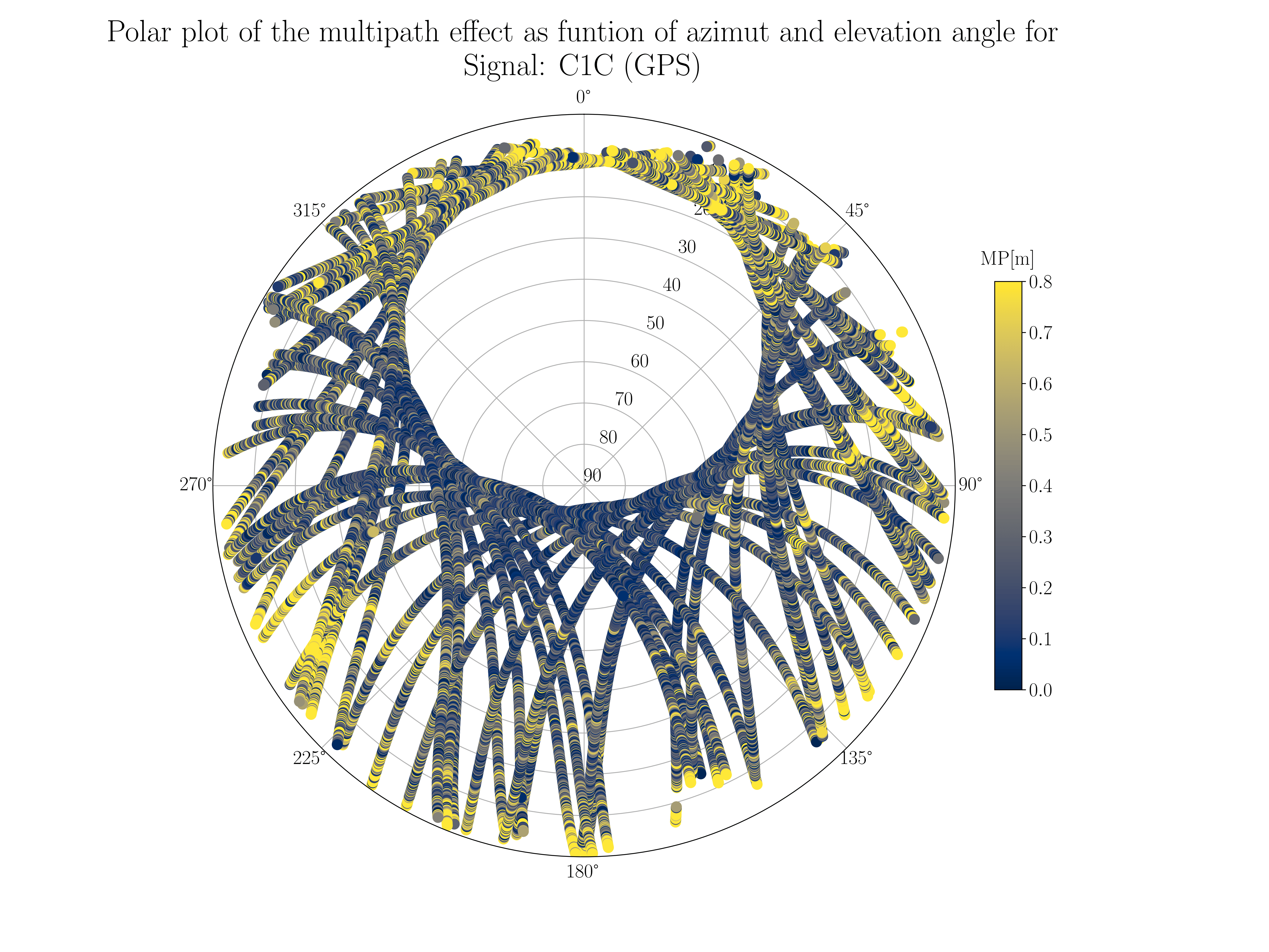
The GNSS_MultipathAnalysis function accepts several keyword arguments that allow for detailed customization of the analysis process. Below is a list of the first five arguments:

rinObsFilename (str): Path to the RINEX observation file (v2.xx, v3.xx, or v4.xx). This is a required argument.
broadcastNav1 (Union[str, None], optional): Path to the first RINEX navigation file. Default is None.
broadcastNav2 (Union[str, None], optional): Path to the second RINEX navigation file (if available). Default is None.
broadcastNav3 (Union[str, None], optional): Path to the third RINEX navigation file (if available). Default is None.
broadcastNav4 (Union[str, None], optional): Path to the fourth RINEX navigation file (if available). Default is None.

More...

sp3NavFilename_1 (Union[str, None], optional): Path to the first SP3 navigation file. Default is None.
sp3NavFilename_2 (Union[str, None], optional): Path to the second SP3 navigation file (optional). Default is None.
sp3NavFilename_3 (Union[str, None], optional): Path to the third SP3 navigation file (optional). Default is None.
desiredGNSSsystems (Union[List[str], None], optional): List of GNSS systems to include in the analysis. For example, ['G', 'R'] to include only GPS and GLONASS. Default is all systems (None).
phaseCodeLimit (Union[float, int, None], optional): Critical limit that indicates cycle slip for phase-code combination in m/s. If set to 0, the default value of 6.667 m/s will be used. Default is None.
ionLimit (Union[float, None], optional): Critical limit indicating cycle slip for the rate of change of the ionospheric delay in m/s. If set to 0, the default value of 0.0667 m/s will be used. Default is None.
cutoff_elevation_angle (Union[int, None], optional): Cutoff angle for satellite elevation in degrees. Estimates with elevation angles below this value will be excluded. Default is None.
outputDir (Union[str, None], optional): Path to the directory where output files should be saved. If not specified, the output will be generated in a sub-directory within the current working directory. Default is None.
plotEstimates (bool, optional): Whether to plot the estimates. Default is True.
plot_polarplot (bool, optional): Whether to generate polar plots. Default is True.
include_SNR (bool, optional): If set to True, the Signal-to-Noise Ratio (SNR) from the RINEX observation file will be included in the analysis. Default is True.
save_results_as_pickle (bool, optional): If True, the results will be saved as a binary pickle file. Default is True.
save_results_as_compressed_pickle (bool, optional): If True, the results will be saved as a binary compressed pickle file using zstd compression. Default is False.
write_results_to_csv (bool, optional): If True, a subset of the results will be exported as a CSV file. Default is True.
output_csv_delimiter (str, optional): The delimiter to use for the CSV file. Default is a semicolon (;).
nav_data_rate (int, optional): The desired data rate for ephemerides in minutes. A higher value speeds up processing but may reduce accuracy. Default is 60 minutes.
includeResultSummary (Union[bool, None], optional): Whether to include a detailed summary of statistics in the output file, including for individual satellites. Default is None.
includeCompactSummary (Union[bool, None], optional): Whether to include a compact overview of statistics in the output file. Default is None.
includeObservationOverview (Union[bool, None], optional): Whether to include an overview of observation types for each satellite in the output file. Default is None.
includeLLIOverview (Union[bool, None], optional): Whether to include an overview of LLI (Loss of Lock Indicator) data in the output file. Default is None.
use_LaTex (bool, optional): If True, LaTeX will be used for rendering text in plots, requiring LaTeX to be installed on your system. Default is True.

Output

analysisResults (dict): A dictionary containing the results of the analysis for all GNSS systems.

Compatibility

Python Versions: Compatible with Python 3.10 and above (tested on 3.10, 3.11, 3.12, and 3.13).
Dependencies: All dependencies will be automatically installed with pip install gnssmultipath.

References

Teunissen, P.J.G. and Montenbruck, O. (eds.), Springer Handbook of Global Navigation Satellite Systems, Springer, 2017. Table 3.4 "Physical parameters of GNSS almanac and ephemeris models", p. 80 — source of the per-constellation $GM$ and Earth rotation rate used for orbit propagation.

License

This project is licensed under the MIT License - see the LICENSE file for details.

Some simple examples on how to use the software:

Run a multipath analysis using a SP3 file and only mandatory arguments

from gnssmultipath import GNSS_MultipathAnalysis

rinObs_file = 'OPEC00NOR_S_20220010000_01D_30S_MO_3.04'
SP3_file    = 'SP3_20220010000.eph'
analysisResults = GNSS_MultipathAnalysis(rinObsFilename=rinObs_file, sp3NavFilename_1=SP3_file)

Run a multipath analysis using a RINEX navigation file with SNR, a defined datarate for ephemerides and with an elevation angle cut off at 10°

from gnssmultipath import GNSS_MultipathAnalysis

# Input arguments
rinObs_file = 'OPEC00NOR_S_20220010000_01D_30S_MO_3.04'
rinNav_file = 'BRDC00IGS_R_20220010000_01D_MN.rnx'
output_folder = 'C:/Users/xxxx/Results_Multipath'
cutoff_elevation_angle = 10  # drop satellites lower than 10 degrees
nav_data_rate = 60  # desired datarate for ephemerides (to improve speed)

analysisResults = GNSS_MultipathAnalysis(rinObsFilename=rinObs_file,
                                         broadcastNav1=rinNav_file,
                                         include_SNR=True,
                                         outputDir=output_folder,
                                         nav_data_rate=nav_data_rate,
                                         cutoff_elevation_angle=cutoff_elevation_angle)

Run analysis with several navigation files

from gnssmultipath import GNSS_MultipathAnalysis

outputdir = 'path_to_your_output_dir'
rinObs = "OPEC00NOR_S_20220010000_01D_30S_MO_3.04_croped.rnx"

# Define the path to your RINEX navigation file
rinNav1 = "OPEC00NOR_S_20220010000_01D_CN.rnx"
rinNav2 = "OPEC00NOR_S_20220010000_01D_EN.rnx"
rinNav3 = "OPEC00NOR_S_20220010000_01D_GN.rnx"
rinNav4 = "OPEC00NOR_S_20220010000_01D_RN.rnx"

analysisResults = GNSS_MultipathAnalysis(rinObs,
                                         broadcastNav1=rinNav1,
                                         broadcastNav2=rinNav2,
                                         broadcastNav3=rinNav3,
                                         broadcastNav4=rinNav4,
                                         outputDir=outputdir)

Run analysis without making plots

from gnssmultipath import GNSS_MultipathAnalysis

rinObs_file = 'OPEC00NOR_S_20220010000_01D_30S_MO_3.04'
SP3_file    = 'SP3_20220010000.eph'
analysisResults = GNSS_MultipathAnalysis(rinObsFilename=rinObs_file, sp3NavFilename_1=SP3_file, plotEstimates=False)

Run analysis and use the Zstandard compression algorithm (ZSTD) to compress the pickle file storing the results

from gnssmultipath import GNSS_MultipathAnalysis

rinObs_file = 'OPEC00NOR_S_20220010000_01D_30S_MO_3.04'
SP3_file    = 'SP3_20220010000.eph'
analysisResults = GNSS_MultipathAnalysis(rinObsFilename=rinObs_file, sp3NavFilename_1=SP3_file, save_results_as_compressed_pickle=True)

Read and work with RINEX observation data

readRinexObs reads the observation file and returns a RinexObsData object holding the observations, epoch times and header information. The correct reader (RINEX v2 or v3/v4) is selected automatically from the version number in the file.

Read a RINEX observation file

from gnssmultipath import readRinexObs

rinObs_file = 'OPEC00NOR_S_20220010000_01D_30S_MO_3.04'
rinex_data = readRinexObs(rinObs_file)

# Every field is available as an attribute
rinex_data.GNSS_obs
rinex_data.time_epochs
rinex_data.approxPosition

The legacy 25-value tuple unpacking is still supported:

GNSS_obs, GNSS_LLI, GNSS_SS, GNSS_SVs, time_epochs, nepochs, GNSSsystems, \
        obsCodes, approxPosition, max_sat, tInterval, markerName, rinexVersion, recType, timeSystem, leapSec, gnssType, \
        rinexProgr, rinexDate, antDelta, tFirstObs, tLastObs, clockOffsetsON, GLO_Slot2ChannelMap, success = \
        readRinexObs(rinObs_file)

Work with the observation data

rinex_data.observations provides a pythonic accessor for retrieving observations by GNSS system, signal code, observation type or frequency band, together with the carrier frequencies needed to form linear combinations.

There are three complementary ways to slice the data:

Slice	Call	Result
one signal, all epochs and satellites	`gps['C1C']`	2-D `[epochs, PRN]`
one signal, one satellite	`gps.sat(23)['C1C']`	1-D over epochs
all signals, one epoch	`gps.epoch(34)`	1-D over PRN per code

Explore what a file contains

from gnssmultipath import readRinexObs

rinex = readRinexObs('OPEC00NOR_S_20220010000_01D_30S_MO_3.04.rnx')
obs   = rinex.observations           # GNSSObservationData

obs.summary()                        # overview of systems, bands and signals
obs.systems                          # ['G', 'R', 'E', 'C']
obs.select(obs_type='L', band=5)     # {'G': ['L5X'], 'E': ['L5X']}
obs.select(system='G', band=1)       # {'G': ['C1C', 'L1C', 'S1C']}

# Per-system accessor, by property or by bracket
gps = obs.gps                        # SystemObservations
gal = obs['E']

gps.codes                            # ['C1C', 'L1C', 'S1C', 'C2W', 'L2W', 'C5X', ...]
gps.pseudorange_codes                # ['C1C', 'C2W', 'C5X', ...]
gps.phase_codes                      # ['L1C', 'L2W', 'L5X', ...]
gps.snr_codes                        # ['S1C', 'S2W', ...]
gps.doppler_codes                    # ['D1C', ...]
gps.bands                            # ['1', '2', '5']
gps.select(obs_type='C', band=1)     # ['C1C']

'C1C' in gps                         # True
gps.n_epochs                         # 2880
gps.n_satellites                     # 37  (max PRN + 1, row 0 unused)
gps.prns                             # observed satellites, e.g. [1, 3, 4, 6, ...]
gps.system_name                      # 'GPS'

Signal metadata and carrier frequencies

sig = gps.signal('L1C')                  # ObsCode
sig.obs_type, sig.band, sig.attribute    # 'L', 1, 'C'
sig.type_name                            # 'phase'
sig.band_description                     # 'L1 (1575.42 MHz)'
sig.frequency(), sig.wavelength()        # 1575420000.0, 0.19029...

gps.signals                              # every code as an ObsCode
gps.frequency('L1C')                     # 1575420000.0
gps.wavelength('L1C')                    # 0.19029...

# GLONASS is FDMA, so its frequencies are satellite specific
obs.glonass.glonass_channel(1)           # 1
obs.glonass.frequency('C1C', prn=1)      # 1602562500.0
obs.glonass.frequency('C1C')             # ndarray indexed by PRN

Retrieve observations

# One signal, all epochs and satellites -> 2-D array [epochs, PRN]
gps['C1C']                           # raw values, missing observations are 0.0
gps.get('C1C')                       # independent copy, missing observations are NaN

# Grouped retrieval -> {code: array}
gps.band(1)                          # {'C1C': arr, 'L1C': arr, 'S1C': arr}
gps.by_type('L')                     # {'L1C': arr, 'L2W': arr, 'L5X': arr}

# One satellite -> 1-D array over epochs
sat = gps.sat(23)
sat.sv_id                            # 'G23'
sat.get('C1C')
sat.frequency('L1C')

# One epoch -> all signals of that epoch (0-based, like the array row index)
ep = gps.epoch(34)                   # epoch(-1) is the last epoch
ep.number, ep.datetime               # 35, numpy.datetime64('2022-01-01T00:17:00')
ep.prns                              # satellites observed in this epoch
ep.get('C1C')                        # 1-D array over PRN
ep.sat(23)                           # {'C1C': ..., 'L1C': ..., ...}
ep.matrix                            # [max_sat, n_codes] block, no copy
ep.to_dataframe()                    # satellites x signals table

gps['C1C'] returns a cached array shared between callers, while gps.get('C1C') always returns an independent copy. Only the codes you actually ask for are built, so a single signal never materialises the full [epochs, satellites, codes] cube.

Loss-of-lock, signal strength and epoch times

# 'S1C' is a normal observable holding the SNR in dB-Hz
gps['S1C']

# .lli and .ss are the single-digit flags appended to each RINEX observation
# record, and are -999 where the field was left blank
gps.lli['L1C']                       # ndarray [epochs, PRN]
gps.ss['L1C']
gps.sat(23).lli['L1C']               # 1-D over epochs
gps.epoch(34).lli['L1C']             # 1-D over PRN

obs.time_epochs                      # [[gps_week, time_of_week], ...]
obs.datetimes                        # ndarray of datetime64 (GPS time scale)
obs.interval                         # 30.0
obs.approx_position                  # ECEF X/Y/Z from the header

Export to pandas

# Long / tidy format: epoch, datetime, sv, prn, code, value
gps.to_dataframe(codes=['C1C', 'L1C'], prns=[1, 3])
gps.to_dataframe(codes=['L1C'], include_lli=True, include_ss=True)
obs.to_dataframe(systems=['G', 'E'], codes=['C1C', 'C1X'])

# Wide format for a single epoch: satellites x signals
gps.epoch(34).to_dataframe(codes=['C1C', 'L1C', 'C2W', 'L2W'])

Use of Pandas DataFrame: one row per satellite and epoch

Pivoting the long frame gives one row per satellite and epoch, with the selected signals as columns. Putting sv first in the index groups and sorts the table by satellite, so all epochs for G01 come first, then G02, and so on:

CODES = ['C1C', 'C2W', 'L1C', 'L2W']

df_gps = (gps.to_dataframe(codes=CODES)
             .pivot(index=['sv', 'datetime'], columns='code', values='value')[CODES]
             .reset_index()
             .rename_axis(columns=None))

df_gps.to_csv('gps_observations.csv', index=False)

    sv            datetime           C1C           C2W           L1C           L2W
0  G01 2022-01-01 00:00:00  2.461555e+07  2.461555e+07  1.293557e+08  1.007966e+08
1  G01 2022-01-01 00:00:30  2.459352e+07  2.459353e+07  1.292399e+08  1.007064e+08

Notes:

A row is kept as long as at least one of the selected codes has a value; a missing individual signal becomes NaN in its own column. Rows are therefore not dropped just because, say, C2W is absent while C1C was tracked.
The table is not n_epochs × n_satellites rows, because satellites rise and set. Pass dropna=False to to_dataframe() for the full rectangular grid.
Sorting on sv works because the identifier is zero-padded (G01…G32), so lexicographic order equals PRN order. Use index=['prn', 'datetime'] if you prefer the numeric PRN in the table instead.
Add prns=[23] to to_dataframe(), or use gps.sat(23).to_dataframe(), to restrict the table to a single satellite.

All systems and all observation codes

Omitting systems and codes includes every constellation and every code in the file. system must be part of the index, since PRN numbers repeat across constellations:

df_all = (obs.to_dataframe()
             .pivot(index=['system', 'sv', 'datetime'], columns='code', values='value')
             .reset_index()
             .rename_axis(columns=None))

df_all.shape        # (101040, 42) for the 30 s OPEC test file

The column set is the union of the codes across the systems, so a code that only exists in one constellation (e.g. C2W for GPS) is NaN for the others. Codes that are declared in the RINEX header but never actually observed are dropped entirely; use obs.to_dataframe(dropna=False) to keep them as empty columns.

Build your own linear combinations

With the arrays and matching carrier frequencies in hand, dual-frequency combinations are a one-liner:

# Ionosphere-free pseudorange
f1, f2 = gps.frequency('C1C'), gps.frequency('C2W')
P1, P2 = gps.get('C1C'), gps.get('C2W')
P_IF = (f1**2 * P1 - f2**2 * P2) / (f1**2 - f2**2)

# Geometry-free phase (ionospheric observable), in metres
L_GF = gps.get('L1C') * gps.wavelength('L1C') - gps.get('L2W') * gps.wavelength('L2W')

The same code works for any system and signal pair:

for system, code1, code2 in [('G', 'C1C', 'C2W'), ('E', 'C1X', 'C5X')]:
    sys_obs = obs[system]
    f1, f2 = sys_obs.frequency(code1), sys_obs.frequency(code2)
    P1, P2 = sys_obs.get(code1), sys_obs.get(code2)
    P_IF = (f1**2 * P1 - f2**2 * P2) / (f1**2 - f2**2)

Carrier frequencies are also available directly:

from gnssmultipath import carrier_frequency, wavelength

carrier_frequency('G', 1)       # 1575420000.0
carrier_frequency('E', 5)       # 1176450000.0
carrier_frequency('R', 1, -4)   # GLONASS G1 on FDMA channel k = -4
wavelength('G', 2)              # 0.24421021...

Read a RINEX navigation file (v2, v3, or v4)

from gnssmultipath import RinexNav

# Works with RINEX v2, v3, and v4 navigation files
rinNav_file = 'BRDC00IGS_R_20220010000_01D_MN.rnx'
navdata = RinexNav.read_nav(rinNav_file, data_rate=60)

Interpolate satellite coordinates to the observation epochs

Satellite coordinates in ECEF can come from two sources, and both are interpolated to the epochs of the observation file:

Source	Class	Typical accuracy	Comment
Broadcast ephemerides (RINEX nav)	`SatelliteEphemerisToECEF`	~1–2 m	Transmitted with the signal, available in real time
Precise orbits (SP3)	`PreciseSatCoords`	~2–5 cm	Downloaded afterwards (e.g. from CDDIS)

Both classes return the same structure:

{'G': {'position': {'1': array([[X, Y, Z], ...]), ...},
       'azimuth':   array([n_epochs, max_PRN + 1]),
       'elevation': array([n_epochs, max_PRN + 1])}, ...}

Both also return coordinates in the ECEF frame at the time of reception, i.e. rotated for Earth rotation during the signal travel time.

Interpolate broadcast ephemerides (RINEX navigation file)

SatelliteEphemerisToECEF converts the broadcast ephemerides to ECEF and propagates them to each observation epoch. For GPS, Galileo and BeiDou the Kepler elements are propagated (Kepler2ECEF), while the GLONASS state vector is integrated with a 4th order Runge-Kutta (GLOStateVec2ECEF).

from gnssmultipath import readRinexObs, RinexNav, SatelliteEphemerisToECEF

rinObs_file = 'OPEC00NOR_S_20220010000_01D_30S_MO_3.04.rnx'
rinNav_file = 'BRDC00IGS_R_20220010000_01D_MN.rnx'

rinex = readRinexObs(rinObs_file)
navdata = RinexNav.read_nav(rinNav_file)

# Approximate receiver position (ECEF) from the observation file header
x_rec, y_rec, z_rec = rinex.approxPosition.flatten().astype(float)

converter = SatelliteEphemerisToECEF(navdata, x_rec, y_rec, z_rec,
                                     desired_systems=['G', 'R', 'E', 'C'])

# Interpolate to the observation epochs (time-of-week in seconds)
tow = rinex.time_epochs[:, 1]
sat_coord = converter.get_sat_ecef_coordinates(tow)

SatelliteEphemerisToECEF accepts either a path to a navigation file, a list of paths, or an already parsed RinexNavData object (as above), which avoids reading the same file twice.

The returned dictionary

sat_coord
└── [system code]            # 'G', 'R', 'E', 'C'
    └── ['position']
        └── [PRN]            # '1', '12'  (string, not zero padded)
            └──> np.ndarray  # shape: (n_epochs, 3), columns X, Y, Z in metres

sat_coord['G']['position']['12']     # ECEF coordinates for G12, shape (n_epochs, 3)

Satellites without ephemerides in the navigation file are None. After compute_satellite_azimut_and_elevation_angle has been called, each system also holds the keys 'azimuth' and 'elevation'.

As a pandas DataFrame

With output_format='pd.DataFrame' the coordinates are returned with a multi-index (timestamp, system, SV) instead of a dictionary. converter.to_dataframe() gives the same result without recomputing.

# Timestamps in, DataFrame out
df_sat_coord = converter.get_sat_ecef_coordinates(rinex.datetimes, output_format='pd.DataFrame')

df_galileo = df_sat_coord.xs('E', level='system')                      # only Galileo
df_e01 = df_sat_coord.xs(('E', 'E01'), level=('system', 'SV'))         # only E01

The time can be given as datetime64 (straight from rinex.datetimes) or as time-of-week. When time-of-week is used, the GPS week is taken from the ephemerides so that the timestamps in the index are still correct.

A single satellite can also be requested directly, which returns (X, Y, Z, dT_rel):

X, Y, Z, dT_rel = converter.get_sat_ecef_coordinates(tow, PRN='G20')

Azimuth and elevation

angles = converter.compute_satellite_azimut_and_elevation_angle(drop_below_horizon=True)

angles['G']['azimuth']      # [n_epochs, max_PRN + 1], indexed by PRN
angles['G']['elevation']

Both arrays are indexed by PRN number, so they can be passed directly to make_skyplot:

import matplotlib.pyplot as plt
import gnssmultipath.plot.make_polarplot as polarplot

gnss_names = {'G': 'GPS', 'R': 'GLONASS', 'E': 'Galileo', 'C': 'BeiDou'}
fig, axes = plt.subplots(2, 2, figsize=(18, 16), subplot_kw={'projection': 'polar'})

for axis, (code, name) in zip(axes.ravel(), gnss_names.items()):
    polarplot.make_skyplot(angles[code]['azimuth'], angles[code]['elevation'], name, None,
                           use_tex=False, save=False, ax=axis)

make_skyplot normally creates its own figure, but with the ax argument it draws into an axis you provide. Font sizes, line widths and the legend are scaled down automatically when ax is given, and saving is skipped since the figure belongs to the caller.

Interpolate precise satellite coordinates (SP3 file)

SP3 files contain precomputed satellite positions in ECEF, typically every 5 or 15 minutes. PreciseSatCoords reads the file (SP3Reader) and interpolates the positions to the observation epochs using Neville's algorithm (SP3Interpolator, 7 points by default).

from gnssmultipath import readRinexObs, PreciseSatCoords

rinObs_file = 'OPEC00NOR_S_20220010000_01D_30S_MO_3.04.rnx'
sp3_file = 'Testfile_20220101.eph'

rinex = readRinexObs(rinObs_file)

# Several SP3 files can also be passed as a list, e.g. to cover a day boundary
precise = PreciseSatCoords(sp3_file, rinex_obs_file=rinex, GNSSsystems=['G', 'R', 'E', 'C'])

# Interpolated coordinates as a DataFrame: Epoch, Satellite, X, Y, Z and Clock Bias
df_precise = precise.satcoords

The class accepts either an already parsed RinexObsData object (as above), a path to an observation file, or just the epochs via time_epochs= if you have no observations:

precise = PreciseSatCoords(sp3_file, time_epochs=rinex.time_epochs, GNSSsystems=['G'])

The receiver position is not needed to interpolate the orbits, only to compute azimuth and elevation, and is therefore an argument to those methods:

receiver_position = rinex.approxPosition.flatten().astype(float)

# Same dictionary structure as for the broadcast ephemerides
sat_data = precise.compute_satellite_azimut_and_elevation_angle(receiver_position,
                                                                drop_below_horizon=True)

sat_data['G']['position']['12']   # interpolated ECEF coordinates for G12
sat_data['G']['azimuth']          # [n_epochs, max_PRN + 1], ready for make_skyplot
sat_data['G']['elevation']

# The angles alone, as a long DataFrame with Epoch, Satellite, Azimuth and Elevation
df_angles = precise.compute_azimuth_and_elevation(receiver_position)

Read in the results from an uncompressed Pickle file

from gnssmultipath import PickleHandler

path_to_picklefile = 'analysisResults.pkl'
result_dict = PickleHandler.read_pickle(path_to_picklefile)

Read in the results from a compressed Pickle file

from gnssmultipath import PickleHandler

path_to_picklefile = 'analysisResults.pkl'
result_dict = PickleHandler.read_zstd_pickle(path_to_picklefile)

Estimate the receiver position based on pseudoranges using SP3 file and print the standard deviation of the estimated position

from gnssmultipath import GNSSPositionEstimator
import numpy as np

rinObs = 'OPEC00NOR_S_20220010000_01D_30S_MO_3.04_croped.rnx'
sp3 = 'Testfile_20220101.eph'

# Set desired time for when to estimate position and which system to use
desired_time = np.array([2022, 1, 1, 1, 5, 30.0000000])
desired_system = "G"  # GPS
gnsspos, stats = GNSSPositionEstimator(rinObsFilename=rinObs,
                                    sp3_file = sp3,
                                    desired_time = desired_time,
                                    desired_system = desired_system,
                                    elevation_cut_off_angle = 15
                                    ).estimate_position()

print('Estimated coordinates in ECEF (m):\n' + '\n'.join([f'{axis} = {coord}' for axis, coord in zip(['X', 'Y', 'Z'], np.round(gnsspos[:-1], 3))]))
print('\nStandard deviation of the estimated coordinates (m):\n' + '\n'.join([f'{k} = {v}' for k, v in stats["Standard Deviations"].items() if k in ['Sx', 'Sy', 'Sz']]))

Estimate the receiver position based on pseudoranges using RINEX navigation file and print the DOP values

from gnssmultipath import GNSSPositionEstimator
import numpy as np

rinObs = 'OPEC00NOR_S_20220010000_01D_30S_MO_3.04_croped.rnx'
rinNav = 'BRDC00IGS_R_20220010000_01D_MN.rnx'

# Set desired time for when to estimate position and which system to use
desired_time = np.array([2022, 1, 1, 2, 40, 0.0000000])
desired_system = "R"  # GLONASS


gnsspos, stats = GNSSPositionEstimator(rinObs,
                                    rinex_nav_file = rinNav,
                                    desired_time = desired_time,
                                    desired_system = desired_system,
                                    elevation_cut_off_angle = 10).estimate_position()

print('Estimated coordinates in ECEF (m):\n' + '\n'.join([f'{axis} = {coord}' for axis, coord in zip(['X', 'Y', 'Z'], np.round(gnsspos[:-1], 3))]))
print('\nStandard deviation of the estimated coordinates (m):\n' + '\n'.join([f'{k} = {v}' for k, v in stats["Standard Deviations"].items() if k in ['Sx', 'Sy', 'Sz']]))
print(f'\nDOP values:\n' + '\n'.join([f'{k} = {v}' for k, v in stats["DOPs"].items()]))

Estimate the receiver's position based on pseudoranges in the desired CRS

Define a specific Coordinate Reference System (CRS) to output the estimated receiver's coordinates. In this case the coordinates will be given in WGS84 UTM zone 32N (EPSG:32632) and ellipsoidal heights.

Note: You can use the EPSG GeoRepository to find the EPSG code for the desired CRS.

from gnssmultipath import GNSSPositionEstimator
import numpy as np


rinObs = 'OPEC00NOR_S_20220010000_01D_30S_MO_3.04_croped.rnx'
rinNav = 'BRDC00IGS_R_20220010000_01D_MN.rnx'

# Set desired time for when to estimate position and which system to use
desired_time = np.array([2022, 1, 1, 1, 5, 30.0000000])
desired_system = "E"  # GPS
desired_crs = "EPSG:32632"  # Desired CRS for the estimated receiver coordinates (WGS84 UTM zone 32N)
gnsspos, stats = GNSSPositionEstimator(rinObs,
                                    rinex_nav_file=rinNav,
                                    desired_time = desired_time,
                                    desired_system = desired_system,
                                    elevation_cut_off_angle = 10,
                                    crs=desired_crs).estimate_position()

print('Estimated coordinates in ECEF (m):\n' + '\n'.join([f'{axis} = {coord}' for axis, coord in zip(['Easting', 'Northing', 'Height (ellipsoidal)'], np.round(gnsspos[:-1], 3))]))

Download GNSS data from CDDIS

The built-in CDDISDownloader class lets you download GNSS data products directly from NASA's CDDIS archive via anonymous FTPS. It supports broadcast navigation files (RINEX v2, v3, v4), observation files, SP3 precise orbit files, and multi-GNSS merged navigation files. Downloaded .gz and .Z files are automatically decompressed.

from gnssmultipath import CDDISDownloader

# Connect using your email (anonymous FTPS login)
with CDDISDownloader(username="your_email@example.com") as dl:
    # Download a RINEX v3 multi-GNSS broadcast navigation file
    nav_file = dl.download_broadcast_nav(year=2022, doy=1, rinex_version=3,
                                         output_dir="./gnss_data/nav")

    # Download a RINEX v4 navigation file (DLR)
    nav_v4 = dl.download_broadcast_nav(year=2023, doy=71, rinex_version=4,
                                       output_dir="./gnss_data/nav")

    # Download a station observation file
    obs_file = dl.download_observation(year=2022, doy=1, station="BRUX",
                                       rinex_version=3,
                                       output_dir="./gnss_data/obs")

    # Download SP3 precise orbit file
    sp3_file = dl.download_sp3(year=2022, doy=1, product="igs",
                               output_dir="./gnss_data/sp3")

    # Download everything for a given day in one call
    bundle = dl.download_daily_data(year=2022, doy=1, station="BRUX",
                                    nav_version=3, include_sp3=True,
                                    output_dir="./gnss_data")

Note: CDDIS uses anonymous FTPS. No Earthdata account registration is needed. A more comprehensive example script is available in src/cddis_download_example.py.

Some background information on implementation

Converting Keplerian Elements to ECEF Coordinates

This section explains step-by-step how satellite positions in Keplerian elements are converted to Earth-Centered Earth-Fixed (ECEF) coordinates. The explanation is showing how the kepler2ecef method has implemented this conversion. This approch works for GPS, Galileo and BeiDou, but not for GLONASS. GLONASS is not storing the satellite positions as Keplerian elements, but uses a state vector instead. The coordinates then get interpolated to the current epoch by solving the differential equation using a 4th order Runge-Kutta.

Steps for Conversion

1. Constants and Inputs

Gravitational Constant and Earth's Mass ($GM$), taken from the ICD of the system the ephemeris belongs to (Teunissen & Montenbruck 2017, Table 3.4, p. 80):

$$ GM = 398,600.5 \times 10^{9} , \text{m}^3/\text{s}^2 \quad \text{(GPS)}, \qquad GM = 398,600.4418 \times 10^{9} , \text{m}^3/\text{s}^2 \quad \text{(Galileo, BeiDou)} $$

Earth's Angular Velocity ($\omega_e $), likewise per system:

$$ \omega_e = 7.2921151467 \times 10^{-5} , \text{rad/s} \quad \text{(GPS, Galileo)}, \qquad \omega_e = 7.2921150 \times 10^{-5} , \text{rad/s} \quad \text{(BeiDou)} $$

Speed of Light ($c$):

$$ c = 299792458 , \text{m/s} $$

Inputs:

Keplerian elements from the RINEX navigation file.
Receiver's ECEF coordinates $(x_\text{rec}, y_\text{rec}, z_\text{rec})$.

2. Calculate Orbital Parameters

Mean Motion ($n_0$):

$$ n_0 = \sqrt{\frac{GM}{A^3}} $$

where $A = a^2 (\text{semimajor axis})$.

Corrected Mean Motion ($n_k$):

$$ n_k = n_0 + \Delta n $$

Time Since Reference Epoch ($t_k$):

$$ t_k = \text{TOW}_\text{rec} - \text{TOE} $$

BeiDou broadcasts $\text{TOE}$ in BeiDou time (BDT), which trails GPS time by 14 seconds, so the reception time is converted before the difference is taken:

$$ t_k = (\text{TOW}_\text{rec} - 14,\text{s}) - \text{TOE} \quad \text{(BeiDou)} $$

$t_k$ is also wrapped to $\pm302,400$ s, so an ephemeris on the other side of a week rollover is propagated over the short arc rather than nearly a full week.

Mean Anomaly ($M_k$):

$$ M_k = M_0 + n_k t_k $$

where $M_0$ is the mean anomaly at reference epoch.

3. Solve for Eccentric Anomaly ($E$):

Use iterative approximation to solve Kepler's equation:

$$ E = M_k + e \sin(E) $$

Repeat until convergence, where:

$$ |E_{\text{new}} - E_{\text{old}}| < \epsilon $$

where $\epsilon$ could be set to $1e-12$

4. Calculate True Anomaly ($\nu$):

Compute $\cos(\nu)$ and $\sin(\nu)$:

$$ \cos(\nu) = \frac{\cos(E) - e}{1 - e \cos(E)}, \quad \sin(\nu) = \frac{\sqrt{1 - e^2} \sin(E)}{1 - e \cos(E)} $$

Use the arctangent to find $\nu$:

$$ \nu = \arctan2(\sin(\nu), \cos(\nu)) $$

5. Compute Orbital Corrections

Corrected Argument of Latitude ($u_k$):

$$ u_k = \nu + \omega + C_{uc} \cos(2u) + C_{us} \sin(2u) $$

Corrected Radius ($r_k$):

$$ r_k = A (1 - e \cos(E)) + C_{rc} \cos(2u) + C_{rs} \sin(2u) $$

Corrected Inclination ($i_k$):

$$ i_k = i_0 + i_\text{dot} t_k + C_{ic} \cos(2u) + C_{is} \sin(2u) $$

6. Longitude of Ascending Node

Account for Earth's rotation:

$$ \Omega_k = \Omega_0 + (\dot{\Omega} - \omega_e)t_k - \omega_e \text{TOE} $$

7. Satellite Position in Orbital Plane

$x$ and $y$ in the orbital plane:

$$ \begin{align*} x &= r_k \cos(u_k) \\ y &= r_k \sin(u_k) \end{align*} $$

8. Transform to ECEF Coordinates

Convert from the orbital frame to the Earth-centered, Earth-fixed frame:

$$ \begin{gather*} X = x \cos(\Omega_k) - y \sin(\Omega_k) \cos(i_k) \\ Y = x \sin(\Omega_k) + y \cos(\Omega_k) \cos(i_k) \\ Z = y \sin(i_k) \end{gather*} $$

BeiDou GEO satellites (C01-C05 in BDS-2 and from C59 in BDS-3) use a different branch of the ICD. The longitude of the ascending node keeps no $-\omega_e t_k$ term, the position is formed in an intermediate frame, and the result is then rotated into CGCS2000:

$$ \Omega_k = \Omega_0 + \dot{\Omega} t_k - \omega_e \text{TOE} $$

$$ \begin{bmatrix} X_k \\ Y_k \\ Z_k \end{bmatrix} = R_z(\omega_e t_k) , R_x(-5^\circ) \begin{bmatrix} X_{GK} \\ Y_{GK} \\ Z_{GK} \end{bmatrix} $$

Applying the MEO equations to a GEO satellite sweeps it around the full orbit instead of keeping it over its station, so this branch is required rather than optional.

9. Relativistic Clock Correction

Account for relativistic effects:

$$ \Delta T_\text{rel} = -\frac{2 \sqrt{A \cdot GM}}{c^2} e \sin(E) $$

10. Earth Rotation Correction (Sagnac Effect)

If the receiver position is known, adjust for the Earth's rotation during signal transmission using an iterative process to correct for the Sagnac effect. The Sagnac effect accounts for the Earth's rotation during the signal's travel time from the satellite to the receiver. This correction ensures that the satellite's position aligns with the time of signal transmission, adjusting for the Earth's rotation.

The Earth's rotation during the signal's travel introduces a positional error if uncorrected. This adjustment ensures high-accuracy satellite positioning and is implemented in the kepler2ecef method part of the Kepler2ECEF class, and the iterative method ensures precise compensation for the Earth's rotation during signal travel time.

The same correction is applied to GLONASS by the correct_for_earth_rotation method of the GLOStateVec2ECEF class, so all four constellations return coordinates in the Earth-fixed frame at signal reception. For GLONASS the interpolated state vector is rotated about the Z-axis by $\omega_e \cdot \text{TRANS}$ instead, since it is not parameterised by $\Omega_k$. Both classes skip the correction when no receiver coordinates are available, because the travel time is then unknown.

Iterative Algorithm for Earth Rotation Correction

Initialize Variables:

$\text{TRANS}_0$: Approximate initial signal travel time, e.g., 0.075 seconds.
$\text{TRANS}$: Variable to store updated travel time.
$j$: Iteration counter.

Iterative Process:

Update the longitude of the ascending node ($\Omega_k$) to account for the Earth's rotation during the signal travel time:

$$ \begin{equation*} \Omega_k = \Omega_0 + (\dot{\Omega} - \omega_e)t_k - \omega_e(\text{TOE} + \text{TRANS}) \end{equation*} $$

Recalculate ECEF coordinates:

$$ \begin{gather*} X = x \cos(\Omega_k) - y \sin(\Omega_k) \cos(i_k) \\ Y = x \sin(\Omega_k) + y \cos(\Omega_k) \cos(i_k) \\ Z = y \sin(i_k) \end{gather*} $$

Compute the distance ($\text{DS}$) between the satellite and the receiver:

$$ \text{DS} = \sqrt{(X - x_\text{rec})^2 + (Y - y_\text{rec})^2 + (Z - z_\text{rec})^2} $$

Update the travel time:

$$ \text{TRANS}_0 = \frac{\text{DS}}{c} $$

Convergence:

Repeat the process until:

$$ |\text{TRANS}_0 - \text{TRANS}| < \epsilon $$

Where $\epsilon$ is a small threshold, e.g., $10^{-10}$. Once the iteration converges, the corrected ECEF coordinates are $X, Y, Z$ and the relativistic clock correction $\Delta T_\text{rel}$.

Interpolating a GLONASS State Vector to ECEF Coordinates

This section explains the steps taken to interpolate GLONASS state vectors using the 4th-order Runge-Kutta method, based on the interpolate_glonass_coord_runge_kutta function provided. The 4th-order Runge-Kutta method is a numerical technique to approximate the solution of ordinary differential equations (ODEs). It iteratively updates the state vector based on the derivatives computed at intermediate steps.

The GLONASS equations of motion describe how the satellite's state (position and velocity) evolves over time under the influence of gravitational and perturbative forces. These equations are differential equations, as they involve derivatives of the satellite's position and velocity.

The state vector $\text{state} = [x, y, z, v_x, v_y, v_z]$ includes the satellite's position ($x, y, z$) and velocity ($v_x, v_y, v_z$). The derivatives of the state vector represent the equations of motion for the GLONASS satellite which include:

Change in Position

$$ \dot{x}, \dot{y}, \dot{z} $$

which equals the velocity components

$$ v_x, v_y, v_z s$$

Change in Velocity

$$ \dot{v_x}, \dot{v_y}, \dot{v_z} $$

depends on:

Gravitational forces.
Perturbations (e.g., due to Earth's oblateness).
External accelerations ($J_x, J_y, J_z$).

1. Inputs

Ephemerides Data: Broadcast ephemerides, including position, velocity, acceleration, and clock corrections, from a RINEX navigation file.
Observation Epochs: Array of observation times, given as GPS week and time of week (TOW).

2. Extract and Convert Ephemeris Data

Read ephemerides parameters for the GLONASS satellite:
- $x_e, y_e, z_e$: Satellite positions at reference time $t_e$ (PZ-90) [km].
- $v_x, v_y, v_z$: Satellite velocities at $t_e$ [km/s].
- $J_x, J_y, J_z$: Acceleration components at $t_e$ $[km/s^2]$.
- $\tau_N$: Clock bias [s].
- $\gamma_N$: Clock frequency bias.

Positions, velocities, and accelerations are converted from kilometers to meters.

3. Time Difference ($\Delta t$)

Convert the reference time $t_e$ from UTC to GPST by adding leap seconds:

$$ t_\text{GPST} = t_e + \text{leap seconds} $$

Compute the time difference between observation and reference epochs:

$$ \Delta t= t_\text{obs} - t_\text{GPST} $$

4. Clock Corrections

Satellite clock error:

$$ \text{clock error} = \tau_N + \Delta t\cdot \gamma_N $$

Clock rate error:

$$ \text{clock rate error} = \gamma_N $$

5. Initialize State Vector

Initial state vector:

$$ state_{vec} = \begin{bmatrix} x_e \\ y_e \\ z_e \\ v_x \\ v_y \\ v_z \end{bmatrix} $$

Initial acceleration vector:

$$ a_{vec} = \begin{bmatrix} J_x \\ J_y \\ J_z \end{bmatrix} $$

6. Runge-Kutta Integration

Time step ($t_\text{step}$): 90 seconds, adjusted based on the magnitude of $\Delta t$.
Iterate using the 4th-order Runge-Kutta method until $\Delta t$ is less than a small threshold (e.g., $10^{-9}$).

Runge-Kutta Equations:

Solving the system of ordinary differential equations (ODEs) using the 4th-order Runge-Kutta method. Runge-Kutta interpolation method implemented in the glonass_diff_eq method apart of the GLOStateVec2ECEF class.

derivatives = glonass_diff_eq(state_vec, a_vec)

this method will be refered to as $f$ from now.

Runge-Kutta steps

Calculate Derivatives: Compute the derivatives using the current state vector and acceleration:

$$ k_1 = f(state_{vec_n}, a_{vec}) $$

$$ k_2 = f\left(state_{vec_n} + \frac{k_1 \cdot t_{step}}{2}, a_{vec} \right) $$

$$ k_3 = f\left(state_{vec_n} + \frac{k_2 \cdot t_{step}}{2}, a_{vec} \right) $$

$$ k_4 = f\left(state_{vec_n} + k_3 \cdot t_{step}, a_{vec} \right) $$

Update State Vector: Compute the updated state vector ($state_{vec_{n+1}}$) as:

$$ state_{vec_{n+1}} = state_{vec_n} + \frac{1}{6} (k_1 + 2k_2 + 2k_3 + k_4) \cdot t_{step} $$

Update Time: Increment the time to the next step:

$$ t_{n+1} = t_n + t_\text{step} $$

Reduce$\Delta t$: Adjust the remaining time difference:

$$ \Delta t = \Delta t - t_\text{step} $$

7. Final Outputs

Position ($x, y, z$) [m]: Extracted from the final state vector.
Velocity ($v_x, v_y, v_z$) [m/s]: Extracted from the final state vector.
Clock Error ($\text{clock error}$) [s]: Calculated during initialization.
Clock Rate Error ($\text{clock rate error}$) [s/s]: Calculated during initialization.

GLONASS Equations of Motion

The derivatives of the state vector ($x, y, z, v_x, v_y, v_z$) are computed as follows:

Radial Distance ($r$):

$$ r = \sqrt{x^2 + y^2 + z^2} $$

Acceleration Terms: Gravitational acceleration:

$$ a_\text{grav} = -\frac{\mu}{r^3} $$

Perturbation due to Earth's oblateness ($J_2$):

$$ a_\text{J2} = 1.5 J_2 \frac{\mu a_e^2}{r^5} \left( 1 - 5 \frac{z^2}{r^2} \right) $$

Equations of Motion:

$$ \dot{x} = v_x, \quad \dot{y} = v_y, \quad \dot{z} = v_z $$

$$ \dot{v_x} = a_\text{grav} x + a_\text{J2} x + 2\omega v_y + \omega^2 x + J_x $$

$$ \dot{v_y} = a_\text{grav} y + a_\text{J2} y - 2\omega v_x + \omega^2 y + J_y $$

$$ \dot{v_z} = a_\text{grav} z + a_\text{J2} z + J_z $$

where:

$\mu = 398,600.4418 \times 10^{9}$ $[m^3/s^2]$ is the gravitational constant.
$J_2 = 1.0826257 \times 10^{-3}$ is the Earth's oblateness factor.
$\omega = 7.292115 \times 10^{-5}$ $[rad/s]$ is the Earth's rotation rate.
$a_e = 6378136.0$ $[m]$ is the semi-major axis of the Earth (PZ-90 ellipsoid).

This method ensures precise interpolation of GLONASS satellite positions and velocities at user-specified epochs.

Interpolating Precise Satellite Coordinates from SP3 file Using Neville's Algorithm

This section explains the steps taken by the SP3Interpolator Python class to compute precise satellite positions from SP3 files. The method leverages Neville's algorithm to perform polynomial interpolation for satellite positions $(X, Y, Z)$ and clock biases at user-specified epochs. The SP3 file is read by the SP3Reader class.

1. Input Data

SP3 Data: Satellite positions $(X_i, Y_i, Z_i)$ and clock biases $\text{Bias}_i$ are provided at discrete epochs $\text{Epoch}_i$. They are extracted from the SP3 file, and the units of the coordiantes are converted from kilometers to meters. The clock bias is converted from microseconds to seconds.
Target Epoch: The observation times ($t$) where interpolation is required. The target epoch is typically the obervation time/epochs from the RINEX observation file.

2. Select Nearest Points

For a given target time $t$:

Compute the time difference:

$$ \Delta t_i = |\text{Epoch}_i - t| $$

Here, $\text{Epoch}_i$ is the time of the $i$-th SP3 entry in seconds. 2. Select the $n$ nearest epochs around the given target time $t$ (e.g., $n=7$) by sorting $\Delta t_i$ in ascending order. By default the number of nearest points for interpolation is set to 7.

3. Apply Neville's Algorithm

Neville's algorithm computes the interpolated value $P(t)$ using $n$ known points $(x_i, y_i)$, where:

$x_i = \text{Epoch}_i$
$p_{i,0}$ is initialized with the satellite data, such as $X_i$, $Y_i$, $Z_i$, or $\text{Bias}_i$.

Recursive Formula

The recursive interpolation formula is:

$$ p_{i,j}(t) = \frac{ (t - x_i) \cdot p_{i+1,j-1}(t) - (t - x_{i+j}) \cdot p_{i,j-1}(t) }{ x_{i+j} - x_i } $$

Where:

$p_{i,0}(t) = y_i$ (initial values) and $j$ is the current degree of the interpolating polynomial.
$t$ represents the target value or interpolation point at which the function $P(t)$ is being approximated.
- In the context of satellite interpolation $t$ is the target epoch or the observation time (in seconds since the reference epoch) for which you are interpolating satellite positions or clock biases. $t$ falls between the nearest known SP3 epochs, $x_i$, and is used for interpolation. $t$ determines the relative weights of the contributions from the known data points $(x_i, y_i)$ to the final interpolated value. For example if you're interpolating the $X$-coordinate of a satellite, $t$ is the observation time at which you want to know the satellite's $X$-position. The algorithm uses $t$ to calculate how much influence each known SP3 epoch $x_i$ and corresponding $y_i$ (satellite's $X$-position at $x_i$) has on the result.
Index $i$ represents the starting point of the interval in the dataset. For example, $p_{i,j}$ corresponds to the interpolated value using points starting from $x_i$.
Index $j$ represents the degree of the polynomial being calculated. $j=0$ corresponds to the initial dataset values ($p_{i,0} = y_i$), while $j=n-1$ represents the final interpolated polynomial.

Algorithm Implementation

Begin with $p_{i,0} = y_i$.
Compute higher-degree polynomials:

$$ p_{i,j}(t) \quad \text{for} \quad j = 1, 2, \dots, n-1. $$

After completing $j = n-1$, the interpolated value is $P(t) = p_{0,n-1}(t)$.

4. Repeat for Each Coordinate component and for the satellite clock bias

Repeat the above steps independently for $X$, $Y$, $Z$, and the clock bias, resulting in $(X, Y, Z, \text{Bias}) \quad \text{at time } t$

Mathematical Summary

Given $n$ nearest points: Let:

$$ p_{i,j}(t) = \begin{cases} y_i & \text{if } j = 0 \\ \frac{ (t - x_i) p_{i+1,j-1} - (t - x_{i+j}) p_{i,j-1} }{ x_{i+j} - x_i } & \text{if } j > 0 \end{cases} $$

The interpolated value is:

$$ P(t) = p_{0,n-1}(t). $$

Example code outlining how Neville's algorithm can be implemented (dummy data)

Click to expand the code

import numpy as np

def interpolate_satellite_data(observation_time, nearest_times, nearest_positions, nearest_clock_biases):
    """
    Interpolates satellite positions and clock bias for a single observation time using Neville's algorithm.

    Parameter:
    ----------
    observation_time : float. Target epoch in seconds (time for which interpolation is required).
    nearest_times : np.ndarray. Array of closest times (epochs) from the SP3 file.
    nearest_positions : np.ndarray. Array of closest satellite positions (X, Y, Z) from the SP3 file.
    nearest_clock_biases : np.ndarray. Array of closest clock biases from the SP3 file.

    Returns:
    -------
    interpolated_position : np.ndarray. Interpolated satellite position (X, Y, Z) at the target epoch.
    interpolated_clock_bias : float. Interpolated clock bias at the target epoch.
    """
    def neville_interpolate(x, y, n):
        """
        Perform polynomial interpolation using Neville's algorithm.

        Parameters:
        ----------
        x : np.ndarray. Differences between nearest times and the target time.
        y : np.ndarray. Satellite data to interpolate (positions or biases).
        n : int. Number of data points.

        Returns:
        -------
        Interpolated value (float)
        """
        y_copy = y.copy()
        for j in range(1, n):
            for i in range(n - j):
                y_copy[i] = ((x[i + j] * y_copy[i] - x[i] * y_copy[i + 1]) / (x[i + j] - x[i]))
        return y_copy[0]

    # Compute time differences relative to the target epoch
    time_diff = nearest_times - observation_time

    # Interpolate satellite positions (X, Y, Z)
    interpolated_position = np.zeros(3)
    for i in range(3):  # Loop over X, Y, Z
        interpolated_position[i] = neville_interpolate(time_diff, nearest_positions[:, i], len(nearest_times))

    # Interpolate clock bias
    interpolated_clock_bias = neville_interpolate(time_diff, nearest_clock_biases, len(nearest_times))

    return interpolated_position, interpolated_clock_bias




if __name__ == "__main__":
	# Example usage on dummy data
	observation_time = 100000  # Example observation time in seconds
	nearest_times = np.array([99990, 99995, 100000, 100005, 100010])  # Example nearest times
	nearest_positions = np.array([
		[1000, 2000, 3000],  # Example X, Y, Z positions
		[1010, 2010, 3010],
		[1020, 2020, 3020],
		[1030, 2030, 3030],
		[1040, 2040, 3040]
	])
	nearest_clock_biases = np.array([0.0005, 0.0006, 0.0007, 0.00008, 0.00009])  # Example clock biases

	interpolated_position, interpolated_clock_bias = interpolate_satellite_data(
		observation_time, nearest_times, nearest_positions, nearest_clock_biases
	)

	print("Interpolated Position (X, Y, Z):", interpolated_position)
	print("Interpolated Clock Bias:", interpolated_clock_bias)

Estimating the Receiver Position Using Least Squares

This section describes how the software estimates the approximate receiver position using pseudoranges and satellite positions through an iterative least-squares adjustment.

Steps for Estimation

1. Inputs

Satellite Positions: The satellite coordinates $(X, Y, Z)$ in ECEF coordinates.
Pseudoranges ($R_{ji}$): The measured distance between the receiver and satellites, corrected for clock errors and relativistic effects.
Initial Receiver Position ($x, y, z$): An approximate starting position for the receiver in ECEF coordinates. Can be set to $(0, 0, 0)$ initially.
Clock Bias ($dT_0$): An initial estimate of the receiver's clock bias.

2. Compute Geometric Range ($\rho$)

For each satellite, compute the geometric distance between the receiver and the satellite:

$$ \rho = \sqrt{(X - x)^2 + (Y - y)^2 + (Z - z)^2} $$

3. Linearization via Taylor Series and Construction of the Design Matrix ($A$)

The observation equation for pseudoranges is non-linear. Before we can use linear algebra, we need to linearize it using a first-order Taylor series expansion. This linearization assumes small corrections to the initial approximate values of $(x,y,z,dT)$. The pseudorange equation is:

$$ R_{ji} = \sqrt{(X - x)^2 + (Y - y)^2 + (Z - z)^2} + dT $$

where $(X, Y, Z)$ are satellite coordinates, $(x, y, z)$ are receiver coordinates and $dT$ is the clock bias. The equation is linearized around an initial guess $(x_0, y_0, z_0, dT_0)$. Using a first-order Taylor series expansion, we get:

$$ R_{ji} \approx R_{ji,0} + \frac{\partial R_{ji}}{\partial x} \Delta x + \frac{\partial R_{ji}}{\partial y} \Delta y + \frac{\partial R_{ji}}{\partial z} \Delta z + \frac{\partial R_{ji}}{\partial dT} \Delta dT $$

where $R_{ji,0}$ is the pseudorange computed at the initial guess. $\Delta x, \Delta y, \Delta z, \Delta dT$ are the corrections to the initial guess. The partial derivatives become:

$$ \frac{\partial R_{ji}}{\partial x} = -\frac{X - x}{\rho}, \quad \frac{\partial R_{ji}}{\partial y} = -\frac{Y - y}{\rho}, \quad \frac{\partial R_{ji}}{\partial z} = -\frac{Z - z}{\rho}, \quad \frac{\partial R_{ji}}{\partial dT} = 1 $$

The design matrix $A$ is constructed using these derivatives:

$$ A = \begin{bmatrix} -\frac{X_1 - x}{\rho_1} & -\frac{Y_1 - y}{\rho_1} & -\frac{Z_1 - z}{\rho_1} & 1 \\ -\frac{X_2 - x}{\rho_2} & -\frac{Y_2 - y}{\rho_2} & -\frac{Z_2 - z}{\rho_2} & 1 \\ \vdots & \vdots & \vdots & \vdots \\ -\frac{X_n - x}{\rho_n} & -\frac{Y_n - y}{\rho_n} & -\frac{Z_n - z}{\rho_n} & 1 \end{bmatrix} $$

This linearized system is solved iteratively, updating $(x, y, z, dT)$ until convergence.

4. Observation Vector ($l$)

The observation vector $l$ represents the difference between the measured pseudoranges and the calculated distances:

$$ l = R_{ji} + c \cdot dT_\text{rel} - (\rho + c \cdot dT_i) $$

5. Normal Matrix ($N$)

The normal matrix is computed as:

$$ N = A^T A $$

6. Correction Vector ($h$)

The correction vector is computed as:

$$ h = A^T l $$

7. Solve for Updates ($\Delta x, \Delta y, \Delta z, \Delta dT_0$)

Solve the linear system:

$$ \Delta \mathbf{x} = N^{-1} h $$

where $\Delta \mathbf{x} = [\Delta x, \Delta y, \Delta z, \Delta dT_0]^T$.

8. Update Receiver Position

Update the receiver's position and clock bias:

$$ x \gets x + \Delta x $$

$$ y \gets y + \Delta y $$

$$ z \gets z + \Delta z $$

$$ dT_0 \gets dT_0 + \frac{\Delta dT_0}{c} $$

9. Iteration

Repeat steps 2–8 until the largest correction in $\Delta \mathbf{x}$ is smaller than a given tolerance ($1 \times 10^{-8}$), or the maximum number of iterations is reached.

Iteration Process in Detail

Initialization: - Start with approximate receiver position $(x, y, z)$ and clock bias $dT_0 = 0$. - Set the improvement threshold and maximum number of iterations.

Convergence Check:

After each iteration, compute the improvement:

$$ \text{improvement} = \max(|\Delta x|, |\Delta y|, |\Delta z|, |\Delta dT_0|) $$

If the improvement is below the threshold, stop the iteration.

Satellite Filtering:

After convergence, filter out satellites with low elevation angles (e.g., $< 15^\circ$).
Recompute the receiver position using the remaining satellites.

Final Outputs

Receiver Position ($x, y, z$): The estimated ECEF coordinates of the receiver.
Clock Bias ($dT_i$): The estimated receiver clock bias in seconds.
Statistical Analysis: Includes residuals, variances, and diagnostics for the least-squares solution.

This iterative least-squares approach ensures high accuracy in estimating the receiver's position while accounting for satellite clock errors and relativistic corrections.

Statistical Parameters of the estimated position

This section describes the key statistical parameters computed during the GNSS positioning process, their significance, and how they are calculated.

1. Residuals ($V$)

Residuals represent the differences between observed and computed values:

$$ V = A \cdot h - l $$

where $A$ is the Design matrix, $h$ is the Adjustments vector and $l$ is the Observations vector. Significance: Residuals indicate the quality of the fit between the observed pseudoranges and the model.

2. Sum of Squared Errors (SSE)

The SSE quantifies the total error in the fit:

$$ \text{SSE} = V^T \cdot V $$

Significance: A smaller SSE indicates a better fit.

3. Standard Deviation of Unit Weight ($S_0$)

The standard deviation of unit weight measures the average residual per degree of freedom:

$$ S_0 = \sqrt{\frac{\text{SSE}}{n - e}} $$

where $n$ is the number of observations and $e$ is the number of unknowns. Significance: $S_0$ is a measure of the model's overall accuracy.

4. Cofactor Matrix ($Q_{xx}$)

The cofactor matrix is computed as:

$$ Q_{xx} = N^{-1} $$

where $N = A^TA$.

5. Covariance Matri ($C_{xx}$)

The covariance matrix is computed as:

$$ C_{xx} = S_0^2 \cdot Q_{xx} $$

Significance: The covariance matrix is crucial for evaluating parameter uncertainties.

6. Dilution of Precision (DOPs)

DOP metrics quantify the geometric quality of the satellite configuration:

Positional DOP (PDOP):

$$ \text{PDOP} = \sqrt{q_X + q_Y + q_Z} $$

Time DOP (TDOP):

$$ \text{TDOP} = \sqrt{q_{dT}} $$

Geometric DOP (GDOP):

$$ \text{GDOP} = \sqrt{\text{PDOP}^2 + \text{TDOP}^2} $$

where $q_X, q_Y, q_Z, q_{dT}$ are the diagonal elements of the cofactor matrix. Significance: Smaller DOP values indicate better satellite geometry and more reliable positioning.

7. Standard Deviations

Standard deviations represent the precision of the estimated parameters:

$$ S_x = \sqrt{C_{xx}[0, 0]}, \quad S_y = \sqrt{C_{xx}[1, 1]}, \quad S_z = \sqrt{C_{xx}[2, 2]}, \quad S_t = \sqrt{C_{xx}[3, 3]} $$

Significance: These values quantify the uncertainty in the estimated receiver coordinates and clock bias.

Computation Workflow

The following steps summarize the computation of these statistical parameters:

Compute Residuals

$$ V = A \cdot h - l $$

Calculate SSE

$$ \text{SSE} = V^T \cdot V $$

Compute $S_0$

$$ S_0 = \sqrt{\frac{\text{SSE}}{n - e}} $$

Derive $Q_{xx}$

$$ Q_{xx} = N^{-1}, \quad N = A^T \cdot A $$

Calculate $C_{xx}$

$$ C_{xx} = S_0^2 \cdot Q_{xx} $$

Extract Cofactors ($q_X, q_Y, q_Z, q_{dT}$) from $Q_{xx}$
Compute DOPs

$$ \text{PDOP}, \text{TDOP}, \text{GDOP} $$

Calculate Standard Deviations

$$ S_x, S_y, S_z, S_t $$

Summary

A comprehensive statistical report includes:

Residuals ($V$): Quantifies model fit.
SSE: Total error.
Standard Deviation of Unit Weight ($S_0$): Average error per degree of freedom.
Covariance Matrix ($C_{xx}$): Absolute parameter precision.
Cofactor Matrix ($Q_{xx}$): Diagonal elements used to compute DOP values.
DOPs: Geometric quality of satellite configuration. Low values indicates good satellite geometry.
Standard Deviations: Uncertainty in receiver coordinates and clock bias.

Name		Name	Last commit message	Last commit date
.devcontainer		.devcontainer
.github/workflows		.github/workflows
.vscode		.vscode
Results_example		Results_example
TestData		TestData
src		src
tests		tests
.gitattributes		.gitattributes
.gitignore		.gitignore
LICENSE.md		LICENSE.md
README.md		README.md
pyproject.toml		pyproject.toml

Latest commit

History

Folders and files

Repository files navigation

GNSS Multipath Analysis

In short

Introduction

Table of Contents

Features

Methodology

Linear combinations

Cycle-slip detection

LLI (Loss of Lock Indicator)

Elevation cutoff and weighting

Coordinate frames, constants and time systems

Installation

Prerequisites

Installing LaTeX (optional)

How to Run It

The steps are:

User arguments

Output

Compatibility

References

License

Some simple examples on how to use the software:

Run a multipath analysis using a SP3 file and only mandatory arguments

Run a multipath analysis using a RINEX navigation file with SNR, a defined datarate for ephemerides and with an elevation angle cut off at 10°

Run analysis with several navigation files

Run analysis without making plots

Run analysis and use the Zstandard compression algorithm (ZSTD) to compress the pickle file storing the results

Read and work with RINEX observation data

Read a RINEX observation file

Work with the observation data

Explore what a file contains

Signal metadata and carrier frequencies

Retrieve observations

Loss-of-lock, signal strength and epoch times

Export to pandas

Use of Pandas DataFrame: one row per satellite and epoch

All systems and all observation codes

Build your own linear combinations

Read a RINEX navigation file (v2, v3, or v4)

Interpolate satellite coordinates to the observation epochs

Interpolate broadcast ephemerides (RINEX navigation file)

The returned dictionary

As a pandas DataFrame

Azimuth and elevation

Interpolate precise satellite coordinates (SP3 file)

Read in the results from an uncompressed Pickle file

Read in the results from a compressed Pickle file

Estimate the receiver position based on pseudoranges using SP3 file and print the standard deviation of the estimated position

Estimate the receiver position based on pseudoranges using RINEX navigation file and print the DOP values

Estimate the receiver's position based on pseudoranges in the desired CRS

Download GNSS data from CDDIS

Some background information on implementation

Converting Keplerian Elements to ECEF Coordinates

Steps for Conversion

1. Constants and Inputs

2. Calculate Orbital Parameters

3. Solve for Eccentric Anomaly ($E$):

4. Calculate True Anomaly ($\nu$):

5. Compute Orbital Corrections

6. Longitude of Ascending Node

7. Satellite Position in Orbital Plane

8. Transform to ECEF Coordinates

9. Relativistic Clock Correction

10. Earth Rotation Correction (Sagnac Effect)

Iterative Algorithm for Earth Rotation Correction

Interpolating a GLONASS State Vector to ECEF Coordinates

1. Inputs

2. Extract and Convert Ephemeris Data

3. Time Difference ($\Delta t$)

4. Clock Corrections

5. Initialize State Vector

6. Runge-Kutta Integration

Runge-Kutta Equations:

Runge-Kutta steps

7. Final Outputs

GLONASS Equations of Motion